Lab Two: Survey of a Sandbox

Introduction

The previous lab was comprised of collecting survey points from a planter plot. In this exercise we learned about different survey techniques. These techniques are: random, systematic, and stratified. For my group’s survey we used a systematic sampling technique with 8 cm intervals. In total there were 180 points measured in a 122 cm by 88 cm rectangular grid. For this lab I went through the process of importing the survey data to ArcMap and editing it for a three dimensional display in ArcScene.

After importing the data, we cleaned it up via normalization. This entailed organizing and analyzing the data to remove redundancies and correct errors.

Each data point collected has three data fields associated with them: an X value, Y value, and a vertical Z value. In this lab we were required to import the Excel data into ESRI ArcMap. This was a simple process of adding the coordinates to map and exporting as a point feature. From here the newly exported feature was opened in ArcScene, a program capable of showing the point data in three dimensions. ArcScene was further utilized as an interpolation tool to improve the display of data via the creation of a 3D raster file. Below I have summarized and given an example of several different interpolation methods available within ArcMap.

For each display I decided to use an oblique angle to best show differences in relief, while maintaining some aspect of scale. One will notice the two scale bars on each map, one labeled “88CM” and the other “122CM.” I have also included a north arrow in each map. It may seem silly to label the distances and orientation for such a small survey area but if someone were unaware of the nature of these past two projects they may not be able to tell the difference between the display of these features in a sandbox to large, kilometer long, features. 

Methods

Figure 1. IDW Interpolation

Inverse distance weighted. This interpolation technique runs on the assumption that features close together are more similar than ones that are further apart which makes this interpolation method useful for large data sets. Due to how the technique weights distances the average number cannot be above or below the highest and lowest points respectively. This makes the display of ridges and valleys a far cry from reality unless the valley bottoms and crests have also been sampled.

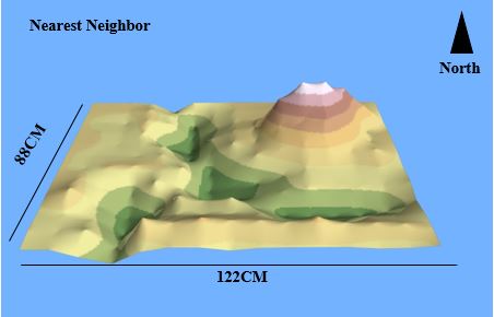Figure 2. Nearest Neighbor Interpolation

Natural Neighbors interpolation, much like IDW, weights the values survey data to create a surface which passes through each point. IDW also will not display un-surveyed valleys or ridges as the displayed surface cannot be more or less that the highest or lowest points.

Figure 3. Kriging Interpolation

Kriging interpolation uses both weighted values and the overall spatial arrangement survey points. The result is a surface that was created from predicted values that strive to emulate unknown values. These values are calculated with the use of clusters and trends in the data. Compared to the other interpolation types Kriging appears to be the most true to form.

Figure 4. Spline Interpolation

Spline interpolation, also known as “thin plate interpolation,” bends a sheet through each point and strives to keep that sheets curvature to a minimum. This creates a smooth, continuous surface.

Figure 5. TIN (Triangular Irregular Network) Interpolation

TIN or triangular irregular network interpolation, works by using each survey point as a node. These nodes are then used to create triangle polygon features that effectively model elevation. Tin files are put to use best with data sets that have a high density of points in areas that have large variations in elevation.

After running all the interpolation methods it was obvious to me that several areas of the landscape needed to be surveyed to better create an accurate representation of the real world sandbox. For example, there was a ridge line on the south edge of the map that appears much lower in the model than it is in the reality. This is due to the spacing of the original survey and how the crest of this ridge line lined up approximately between the survey distances, meaning that only the lower sides were measured.

Figure 6. Locations of new survey points (North is down).

My group did a second, much less extensive, survey of the micro landscape that included 17 new points that were collected in the most problematic areas of the original survey (Figure 6).

Figure 7. TIN interpolation showing the effects of additional survey points to underrepresented areas. Note that the ridge crest on the southern edge of the map is displayed with a higher altitude and appears more peaked than the previous TIN image. 

I added the new survey points in the same fashion as the first set of data. From here it was a simple process to merge both data sets, open them in ArcScene, and create a TIN file using the same interpolation method as before (Figure 7).

Summary and Conclusions

When compared to other field based surveys I would have to say that this example is relatively realistic, aside from how we had the ability to resurvey the landscape. In a full scale survey of a large landscape it is often likely that resurveying an area is not possible. 

It is not always possible to perform such a detailed grid-based survey. In many cases the terrain is far too rough and inaccessible to perform such a survey on the ground. With remote sensing technology as it is today it is fairly easy, if expensive, to get very accurate measurements of landscapes.

Interpolation methods such as those used here are commonly used to display temperature data, rainfall amounts, and, in the field of remote sensing, image rectification.